
Formulas, Functions, and AutoFill
Operators
All Excel formulas begin with an equals sign (=). Operators define the actions within your formula, following the standard algebraic order of operations:
- Parentheses ( ): Perform operations inside first.
- Exponentiation (^): Raise a number to a power.
- Multiplication (*): Calculate the product.
- Division (/): Calculate the quotient.
- Addition (+): Calculate the sum.
- Subtraction (-): Calculate the difference.
Formulas
- Select the desired cell.
- Start with an equality sign (=).
- Insert your expression and press Enter to calculate.
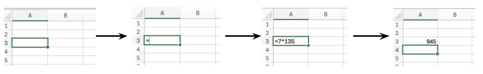
Example: set A3 equal to the product of 7 and 135. Press enter to calculate the value.
- cell A3 is highlighted
- cell A3 has a = in it
- cell A3 has =7*135
- cell A3 has the number 945 (the product of 7*135)
Cell Referencing
Users can reference data from a cell or range of cells for calculations. Each cell has a unique reference (e.g., A3 for the value 945). Cell references can be substituted in formulas for values.
Example:
Repeat the previous example using the values from above. Insert 7 in cell A1 and 135 in cell A2.
- cell A1 has the number 7 and cell A2 has the number 135
- cell A3 now has =A1*A2
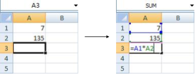
Insert “=A1*A2” to create a formula using cell referencing instead of inserting “=7*135” in A3.
Note: the reference points to the cell and not the value inside. A1 tells Excel to look at A1 and pull whatever value it holds. If you update the value of A1 (e.g., from 7 to 9), then it updates all the calculations. A1 does not tell the calculator to look for the value 7.
Example:
Change the value of A2 to 123.
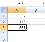
The value of A3 has changed to 861, but the formula of the cell is still A1*A2.
Referencing
Data can be referenced from the same sheet or different sheets:
- Same Sheet:
=A2(relative reference)=$A$2,=A$2,=$A2(absolute references) The$symbol in absolute references locks the column, row, or both, preventing them from changing when a formula is autofilled or copied.
- Another Sheet:
=Sheet1!A2=Name!A2(for named sheets)
Functions
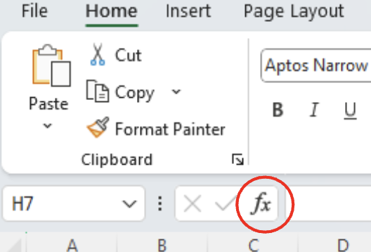
Excel offers many built-in functions that operate on a range of cells. You can access these functions by:
- type in the equals (=) sign followed by the name of the function
- click the fx button next to the cell value bar, or
- find the sigma (Σ) symbol dropdown arrow in the Editing section of the Home ribbon.

Referencing a Range of Cells: Specify a starting and ending cell for continuous ranges, or list individual cells for non-continuous ranges.
- A1:A4 includes A1, A2, A3, and A4.
- A1:B3 includes A1, A2, A3, B1, B2, and B3.
A1:A3, C1:C3 includes A1, A2, A3, C1, C2, and C3.
Common Functions:
- =SUM(range) finds the sum of a range of values
- =AVERAGE(range) finds the average of a range of values
- =MIN(range) finds the smallest value in a range
- =MAX(range) finds the largest value in a range
- =COUNT(range) counts the number of cells in a range when the range contains numbers
- =COUNTA(range) counts the number of cells in a range when the range contains any kind of data
Conditional Functions
Conditional functions perform calculations only if specified criteria are met. These functions test a range and proceed based on whether the condition is TRUE or FALSE. Conditions can be any relational comparison:
Examples:
- A3>14 if the value of cell A3 is larger than the number 14
- D5<=2 if the value of cell D5 is less than or equal to the number 2
- T47=”cheese” if the value of cell T47 is “cheese”
We’ll cover AND, OR, IF, COUNTIF, and SUMIF, along with nested IF statements.
AND
=AND(condition1, [condition2], …)
AND will evaluate to TRUE only if all conditions are true.
For example,
=AND(G2=”BLAH”,A2=”OCHO”)
will evaluate to TRUE if the cell G2 is “BLAH” and the cell A2 is “OCHO”.
OR
=OR(condition1, [condition2], …)
OR will evaluate to TRUE if any of the conditions are true.
For example,
=OR(E2>12,F2<54)
evaluates to TRUE if E2>12, or F2<54, or if both of the conditions are true!
IF
=IF(condition,value_if_true,value_if_false)
If the given condition is true, the cell will be set to the “value_if_true.” If the condition is false, the cell will be set to the “value_if_false.” The “value_if_false” is an optional input, which defaults to FALSE.
Example:
=IF(A2>3,32,”Number too small”)
Reads: If A2>3 is true, then set the cell to 32. Otherwise, set the cell to “Number too small”
Nested IF Functions
Multiple IF functions can be nested to test for multiple conditions.
Example:
Test the condition of whether the contents of cell A2 are between 10 and 20.
=IF (A2>20,”Number too large”, if (A2<10,”Number too small”, “Just right!”))
If it the value of A2 is larger than 20, the active cell will be set to “Number too large.” If A2 is less than 20, it will be tested to see if the value of A2 is less than 10. If it is, the active cell is set to “Number too small.” Otherwise, we know that the value of A2 must be between 10 and 20, so the active cell is set to “Just right!”
COUNTIF
=COUNTIF(range,criteria)
The “countif” function will increment the active cell by one each time the criteria is true for a cell in the given range.
Example:
In column F you have colors, and want to count the number of occurrences of “red”.
=COUNTIF (F1:F230, “=red”)
If a cell in F1:F230 satisfies “=red”, then increment the active cell by one.
SUMIF
=SUMIF(range,criteria,sum_range)
The “SUMIF” function takes a range and a corresponding sum_range of the same size. Each time the criteria is true, the value in the cell for sum_range gets added to the active cell. If “sum_range” is not specified, excel will treat “range” as “sum_range” as well.
Example:
You wish to know how many hours you have spent watching television, from a database of your time spent on various activities.
=SUMIF (D1:D230,”=television”, H1:H230)
If a cell in D1:D230 satisfies “=television”, then increment the active cell by the corresponding cell from H1:H230. If cell D7 contains the word “television,” the active cell will be incremented from the corresponding cell from H1:H230, or cell H7.
Autofill and Referencing
Autofill quickly copies formulas or data following a pattern.
Basic Autofill (Click-and-Drag):
- Select a cell with a value or formula (e.g., =A1+1).
- Hover over the small square (fill handle) in the bottom-right corner.
- Click and drag over the cells you want to fill.
- Release the mouse to apply the pattern. Excel will detect patterns (numbers, weekdays, formulas) and continue them.
Example:
Enter a value in the A1 cell. In the cell below it, enter the formula: =A1+1. If A2 has =A1+1, dragging down will increment each row (and cell reference).
Use the autofill feature and drag the formula down a few cells. Select cell A3. It now contains the formula: =A2+1
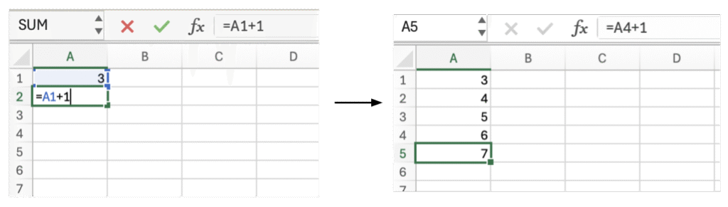
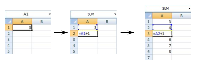
Relative Referencing: When autofilling, cell references change relative to their new position. For instance, dragging a formula =A1+1 from A2 down to A3 will change it to =A2+1.
A3 will reference A2, and A4 will reference A3, and so on. Autofill will follow this formatting horizontally as well. Autofill again, and select A3. Notice how A3 is now referencing A1.
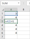
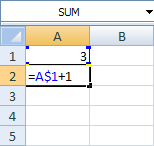
Absolute Referencing: To maintain a constant reference during autofill, use a dollar sign ($) between the column and row (e.g., =A$1+1). This makes the reference absolute, so dragging =A$1+1 from A2 to A3 will keep the reference as A$1. In other words, (A1 vs A$1) affects how formulas are copied. In this case, you are staying in column A so we don’t need to write $A also. If you drag across columns, you would need to write $A.
Double-Click Autofill: If you’re working in a column with adjacent data, double-clicking the fill handle will autofill downward until it reaches an empty row.
Tip: Autofill works in any direction (down, up, left, or right). Remember that how formulas are copied is affected by whether data is statically referenced (A1) or cell addressed (A1).